A few days ago I tried running Gemma 4 26B-A4B on my M1 MacBook Air (16 GB) using TurboFieldfare. On paper it has no business working on this laptop: even at 4-bit, the weights alone are about 14 GB, before you count the OS and the KV cache. Yet TurboFieldfare reports a resident set of about 2.5 GB while serving the model. I wanted to know how. The answer turned out to be an old friend: the database buffer pool.
A few terms come up a lot below. If any of this is new, refer to the glossary at the end for quick 1 line definitions.
The trick: it’s a Mixture-of-Experts model
The answer is in the architecture. The Gemma 4 26B-A4B is a Mixture-of-Experts (MoE) model that activates only ~4 billion parameters per token, delivering performance nearly identical to its heavier 31B dense sibling. The architecture uses a vertical stack of 30 consecutive layers, where each layer houses its own local pool of 128 specialized experts and dynamically routes just the top 8 experts per token. To capture broad, foundational logic, a single shared expert also runs constantly alongside these dynamic expert pools in every single layer.[]
In a normal deployment, all of them still sit in RAM. TurboFieldfare doesn’t do that. It keeps only the dense core resident (embeddings, attention, the router, and the shared expert about 1.35 GB) plus the KV cache. Of the routed experts, it holds just a small per-layer cache in memory (16 per layer by default, evicted least-frequently-used), while the full 12.9 GB routed-expert pool lives on SSD. When the router picks an expert that isn’t cached, the runtime reads it off disk on the spot. On my machine the resident set sat around 2.5 GB.
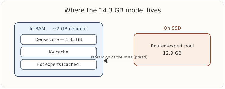
The resident core and a small expert cache stay in RAM; the full routed-expert pool streams from SSD on demand.
The trade-off is that an expert not already in memory has to come off disk first, and SSD latency is much higher than RAM latency.
This isn’t an idea TurboFieldfare invented; offloading inactive experts is an active area of ML systems research. What caught my attention wasn’t the novelty but how cleanly the design maps onto something I already understood from a completely different area, and how it makes a model this size run on consumer hardware.
Where I’d seen this before
This is the point where it clicked. Swap the vocabulary and you’re describing a database buffer pool.
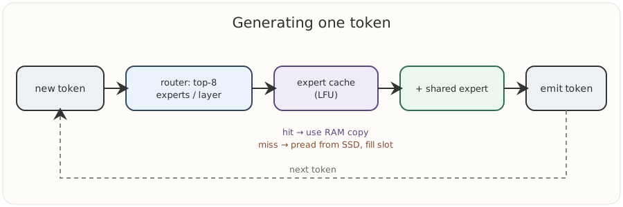
Each token: the router selects experts, the cache serves hits and streams misses from SSD, then the shared expert’s output is added in.
| Database | TurboFieldfare |
|---|---|
| Table pages on disk | Expert weights on SSD |
| Buffer pool | Resident expert cache |
| Page fault | Expert fetch from SSD |
| Buffer pool size | Number of resident slots |
A database doesn’t drag an entire table into memory. It keeps the hot pages in the pool, faults the rest in from disk on demand, and evicts as it goes. TurboFieldfare is doing the same thing, one abstraction level up, with expert weights instead of pages.
The analogy runs deeper than the surface mapping. Lot of databases manages their own buffer pool rather than just mmap-ing their data files and letting the OS page cache decide what to keep. Because the OS doesn’t know which pages matter, and its eviction tends to fight the database’s access pattern. TurboFieldfare’s optimization log describes hitting exactly that wall. The first streaming design mmap-ed the expert pool and let demand paging fetch experts, which looked clean due to no explicit copies. But the laptop couldn’t keep the cold working set warm, and a cold expert read cost about 9.9 ms through demand paging versus about 2.8 ms through an explicit pread (a direct, offset-based file read). End to end, that was the difference between roughly 0.5 and 4 tokens/sec. The fix was to stop leaning on the OS and manage an explicit, bounded per-layer expert cache with its own reads. That’s the same conclusion databases reached decades ago.
There’s a second layer to the analogy I almost missed. A buffer pool decides what stays resident; it doesn’t by itself hide the cost of a miss. TurboFieldfare hides misses by running the shared-expert branch in parallel with the expert reads, so the GPU has work to do while the SSD catches up. Databases do the same with prefetching the next set of pages from disk in advance. The cache determines what you read; the overlap determines whether the wait shows up in your token rate.
It isn’t a perfect mapping. A database’s hot set is fairly stable, so the pool settles into a steady working set. An MoE router can pick a different mix of experts on almost every token, so the working set is choppier and the cache has to work harder. But the systems thinking is the same.
Trying to make it faster
I was getting around 5 tokens/sec on the M1 Air. That’s too slow for live chat, but perfectly fine for the async things I actually reach for it: reviewing code, summarizing documents, working through an unfamiliar codebase, asking architecture questions.
One caveat before you get excited: that number is decode pass speed, once generation is rolling. The first token involves a prefill pass over the whole prompt, and prefill is where this runtime is slowest, close to a minute for a ~1,000 token prompt.
Naturally I tried to push it. The runtime defaults to a 16 slot LFU cache per layer; I’d already been running with the cap raised to 24, and the logic for going further seemed obvious: more resident experts, fewer SSD reads, faster generation. So I bumped it to 32.
Throughput went the wrong way, from about 5 to 4.5 tok/s, and resident memory climbed roughly a gigabyte.
Before blaming the inference engine, I looked at what the OS was doing:
Physical Memory : 16 GB
Memory Used     : 15 GB
Compressed      : 5.5 GB
Swap Used       : ~1 GB
Unused          : 200 MB
Most likely explanation: Compressed memory is RAM that macOS has squeezed to make room; swap is RAM spilled onto disk. Both are signs the system is under pressure. My hypothesis is that the memory manager spent more than the streaming layer saved, trading a few avoided SSD reads for a system quietly paging. The details support that read: LFU with more slots keeps more rarely-used experts resident, so the hit rate barely improves while the footprint grows, and the extra buffers give the OS more to squeeze. I didn’t isolate swap as the sole cause here, but the shape of the failure matches something familiar: an over-sized database buffer pool on a box that starts swapping. Bigger cache, slower system.
Final Config
After a few rounds I settled back on 24 resident expert slots, an 8K–16K context, temperature 0.2, Top-K 32, Top-P 0.95. There was no secret setting that doubled the throughput, just the point where the hardware stayed balanced.
Takeaways
The thing I’ll remember from this isn’t the half-token-per-second tuning. It’s that the ideas making local MoE inference feel like magic: working sets, caching, eviction, virtual memory. TurboFieldfare is a genuinely clever piece of engineering, but it’s clever within a lineage, and knowing the older ideas is what made the new one legible to me.
Honestly, I find that more interesting than the headline fact that a 26B MoE model can run on a fanless laptop in a couple of gigabytes of RAM. Though that’s still a very good trick.
Glossary
- Mixture-of-Experts (MoE): an architecture split into many small sub-networks (“experts”), where a router activates only a few per token instead of running the whole model.
- Resident expert: an expert whose weights are currently loaded in RAM, ready to use without a disk read.
- Weights: the learned numbers that make up a model; “loading the model” means loading these into memory.
- KV cache: stored results from earlier tokens so the model doesn’t recompute the whole conversation on every new word.
- Temperature: how predictable vs. varied word choice is; low is focused, high is more random.
- Top-K: only consider the K most likely next words when generating.
- Top-P: only consider the smallest set of next words whose combined probability reaches P.
pread: a system call that reads bytes from a specific point in a file directly, without scanning through it first.
References and Further Reads
- TurboFieldfare: source, README, and architecture notes
- TurboFieldfare: the experiments that shaped the runtime (
mmapvspread, the LFU expert cache) - Maarten Grootendorst: A Visual Guide to Gemma 4
- Google: Gemma 4 model overview
Opined and edited by me, drafted and visualised with AI. © Shahbaz Ahmed, 2026. Shared under CC BY 4.0 — use it, adapt it, just credit it.